Impedance-based stability analysis: Putting It All Together

The last article of the series on impedance-based stability analysis

In 2015, engineers from the German TSO TenneT stood in front of a conference audience in Bonn and described something that was not supposed to happen. BorWin1 — the world’s first HVDC-connected offshore wind farm — had developed sustained electrical oscillations at several hundred hertz. Nothing had failed. Every component worked exactly as designed. The planning studies, done with the industry’s standard tools, had shown no problem at all. And yet the system oscillated, persistently enough to damage equipment, for reasons none of the standard tools could see.

The cause, when it was finally understood, was not a faulty component. It was an interaction — the converter’s control system and the offshore cable network forming a feedback loop that none of the classical, machine-era stability methods were built to analyse. The tools that eventually explained it, and fixed it without touching a single piece of hardware, came from a different tradition entirely: the frequency-domain, impedance-based methods this series has spent seven articles building.

This final article is free, and deliberately so, because it is the map. Everything the series has built — the feedback-loop insight, the Nyquist verdict, the Bode margins, the scanning methods, the limits, and the passivity guarantee — assembled into one picture, with a practical guide to which tool answers which question. If you have read the whole series, this is your synthesis. If you are arriving here first, this is what the journey looks like from the summit — and every stage of it is one article away.

Eight articles, one journey

The series was built as a single argument, each article resting on the one before. Laid end to end, it runs from a question to a guarantee.

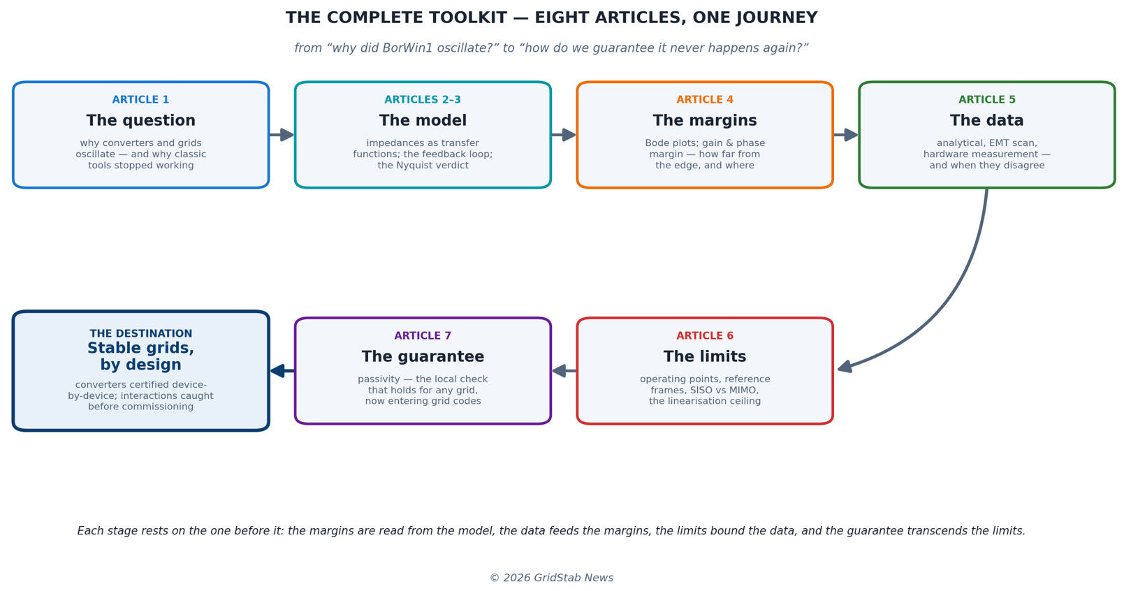
Figure 1. The complete toolkit in one map. The question (why converters and grids oscillate) leads to the model (impedances in a feedback loop), the model to the verdict and margins (Nyquist and Bode), the margins to the data that feeds them (frequency scans), the data to its limits — and the limits, finally, to the guarantee that transcends them (passivity). Each stage is one article of the series.

It begins with the question. Article 1 laid out why the grid’s stability problem changed character: synchronous machines obey physics that is fixed and known, while converters obey control code that is proprietary, fast, and different in every product — the white-box problem that shadows everything that follows. The classical toolset assumed the machine era. The events of the last decade, BorWin1 among them, are what happened in the gap.

Then the model. Articles 2 and 3 rebuilt the problem in the frequency domain: every device reduced to an impedance — a transfer function measurable from its terminals, no access to the control code required — and the converter–grid pair revealed as a feedback loop whose loop gain is simply the ratio of the two impedances. That reframing, from Middlebrook’s classic input-filter work, is what makes the whole field possible. On top of it sits the Nyquist criterion, the 1932 test that reads stability straight off the two curves: does the loop gain encircle −1, or not.

Then the quantities. A verdict is not enough for engineering; Article 4 added the Bode plot and its two famous numbers — gain margin and phase margin — which turn “stable or not” into “how far from the edge, and in which frequency band.” It closed with the BorWin1 post-mortem: the two impedance curves crossing in the band where the real oscillations were measured, with a phase margin that was not thin but negative. The event that opened the series became a worked example.

Then the data. Margins are only as good as the impedance curves behind them, and Article 5 covered the three ways those curves are actually obtained — analytical derivation when you own the design, EMT frequency scanning of the vendor’s black-box model when you don’t, and hardware measurement when you need ground truth — along with the uncomfortable fact that the three methods disagree exactly where it matters most, at high frequency.

Then the honesty. Article 6 mapped the edges of the method: the impedance is a snapshot valid at one operating point, not a portrait of the device; the reference frame you choose changes what you can see; the converter is a 2×2 matrix that only sometimes collapses safely to a single number; and the entire framework is linear in a world where the worst events — faults, trips, loss of synchronism — are anything but. Knowing these limits is what separates using the method from being used by it.

And then the destination. Article 7 introduced passivity: if the real part of a converter’s impedance never goes negative, the converter can only absorb energy — and a device that cannot supply energy cannot feed an oscillation, in any grid, at any operating point, next to anything. It is a condition checkable on the converter alone, it survives every change that forces the margin approach back to square one, and it is already appearing in real grid codes. It does not replace the toolkit; it is where the toolkit was heading all along.

Which tool, when

Synthesis is only useful if it changes what you do on Monday morning. In practice, nearly all of connection engineering reduces to four questions — and each has a right tool.

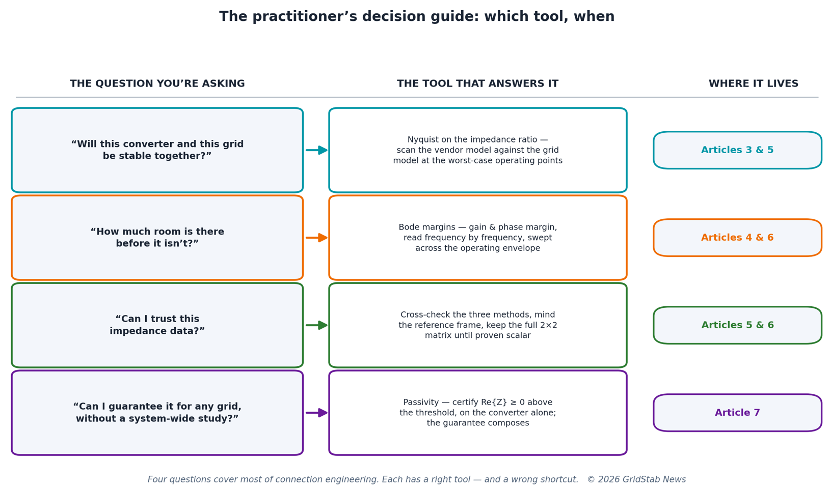
Figure 2. The practitioner’s decision guide. Four questions cover most of the stability work in a connection project; each maps to a specific tool and a specific place in the series. The common failure mode is answering one question with the tool that belongs to another.

The first question — will this converter and this grid be stable together? — is the classic connection-study question, and it belongs to the Nyquist test applied to scanned impedances. The craft is not in the criterion but in the inputs: scanning the vendor model at the worst-case operating points, not just the convenient ones, because the operating point you skip is the one where the instability lives.

The second — how much room before it isn’t? — belongs to the Bode margins, read frequency by frequency and swept across the operating envelope. Margins are what turn a stability study into an engineering conversation: they tell the designer which band is fragile, the TSO how much grid change the connection can absorb, and both sides how much headroom a firmware update may consume.

The third — can I trust this impedance data? — is the question most often skipped. Cross-check the methods where they overlap; be explicit about the reference frame; keep the full 2×2 matrix until the coupling terms are proven small, and expect them to matter most in the low-frequency band where the PLL lives. The most expensive words in this field are “the model said it was fine.” BorWin1’s planning studies said exactly that.

And the fourth — can I guarantee it for any grid, without a system-wide study? — has exactly one honest answer, and it is passivity. It is conservative; it will reject some aggressive designs that would have survived. That is the price of a guarantee that composes: passive plus passive is stable, whoever built the converters and whatever grid they land in.

What this means, depending on where you sit

If you develop or operate generation assets: the impedance study is moving from an exotic annex to the critical path of your connection agreement. The developers who treat the EMT model and its impedance scan as first-class deliverables — procured early, validated against measurement, swept across the envelope — are the ones who connect on schedule. The ones who treat it as paperwork discover, late, that the model is the project.

If you build converters: your impedance is becoming your public interface. Grid codes are beginning to specify how it must behave — Great Britain’s GC0137 already assesses grid-forming capability through passive-impedance behaviour across 5 Hz to 1 kHz, and AEMO’s specification asks for a positive-real impedance across the sub-synchronous range. The control levers that shape the impedance — delay compensation, active damping, virtual resistance — are no longer internal tuning details. They are compliance.

If you plan or operate the network: the toolkit is what makes converter-dense operation tractable, but only if the burden is shared sensibly. The emerging pattern — converters certified passive above a threshold, the network kept free of weakly damped resonances below it — splits the problem between the parties who can actually control each half. The railway sector has now codified exactly this structure in EN 50388-2, published in 2025 for AC traction systems; the pattern it formalises is the one the wider grid is converging toward.

And if you invest in or regulate this sector: oscillatory stability has quietly become a gating item for the energy transition. Every gigawatt of wind, solar, storage, and HVDC arrives through a converter, and the grid’s ability to absorb them is bounded not by energy but by interactions. The jurisdictions writing impedance and passivity requirements into their codes now — Britain first among them, with regulatory approval of its grid-forming specification in January 2022 — are the ones deciding how fast their queues can move.

Where the field goes from here

Three trajectories are visible from where this series ends. First, the toolkit is becoming compulsory literacy. TSOs increasingly require full EMT models and impedance characterisation as connection conditions; what was research a decade ago is boilerplate in connection agreements today. Second, the centre of gravity is shifting from analysis to specification — from “study each connection” to “specify the impedance behaviour every device must present,” which is passivity’s territory, and the reason it is moving from academic elegance into grid codes. Third, grid-forming converters change the questions but not the framework: a grid-forming control presents a different impedance — often a friendlier one — but it is still an impedance, still scannable, still boundable by the same margins and the same passivity condition. The toolkit in Figure 1 is not a snapshot of current practice. It is the durable structure underneath it.

The honest caveat from Article 6 still stands, and always will: this is small-signal machinery. It tells you whether every operating point is locally stable and how robustly; it does not tell you whether the system survives the journey between operating points when a fault throws it across the map. Large-signal EMT simulation and the small-signal impedance toolkit are complements, not rivals — the connection studies that catch everything use both.

The complete series

This finale is free. The six deep dives beneath it — the full derivations, the figures, the case studies, and the practical detail that this synthesis can only gesture at — are for paid subscribers of GridStab News.

IMPEDANCE-BASED STABILITY ANALYSIS — THE SERIES

Article 1 — Why Impedance, Why Now. The white-box problem, the events that broke the classical toolset, and why the frequency domain is the answer. Free.

Article 2 — From Time Domain to Transfer Functions. The same system, two languages — and the perturb-and-measure idea everything else is built on.

Article 3 — The Nyquist Stability Criterion. The hidden feedback loop, the −1 point, and the 90-year-old test that reads stability off two curves.

Article 4 — Reading Bode Plots. Gain margin, phase margin, what “good” looks like — and the BorWin1 post-mortem with a negative phase margin exactly where the oscillations were measured.

Article 5 — Frequency Scan Techniques. Analytical, EMT scan, hardware measurement — and why the three methods disagree exactly where it matters.

Article 6 — The Limits of Frequency Scans. Operating points, reference frames, the SISO trap, and what linearisation can never see.

Article 7 — Passivity: The Elegant Shortcut. The local check with the global guarantee — and where it already sits in real grid codes.

Become a paid subscriber to unlock all seven — and everything GridStab News publishes next

Thank you for reading the series. — Gilles

© 2026 GridStab News. All rights reserved.