
Frequency Scan Techniques
Article 5 in the series on impedance-based stability analysis

Over the first four articles in this series, we have built a complete conceptual toolkit for impedance-based stability analysis. Transfer functions (Article 2), the Nyquist criterion (Article 3), and Bode plots with gain and phase margins (Article 4) together give us a framework for deciding, quantitatively and frequency by frequency, whether a converter and a grid will coexist stably at a given connection point.
But every Nyquist plot, every Bode plot, and every stability margin we have discussed rests on one assumption: that the impedance curves feeding those tools actually exist — that someone, somewhere, has produced them. An impedance curve does not fall from the sky. It must be obtained, and the method by which it is obtained determines what it captures, what it misses, and how far it can be trusted.
This article is about the practical question that sits beneath all the theory: how do you actually get the impedance data?
Three methods, one output
There are three fundamentally different ways to obtain the impedance of a converter or a grid segment, and they correspond to three levels of access to the device under study.
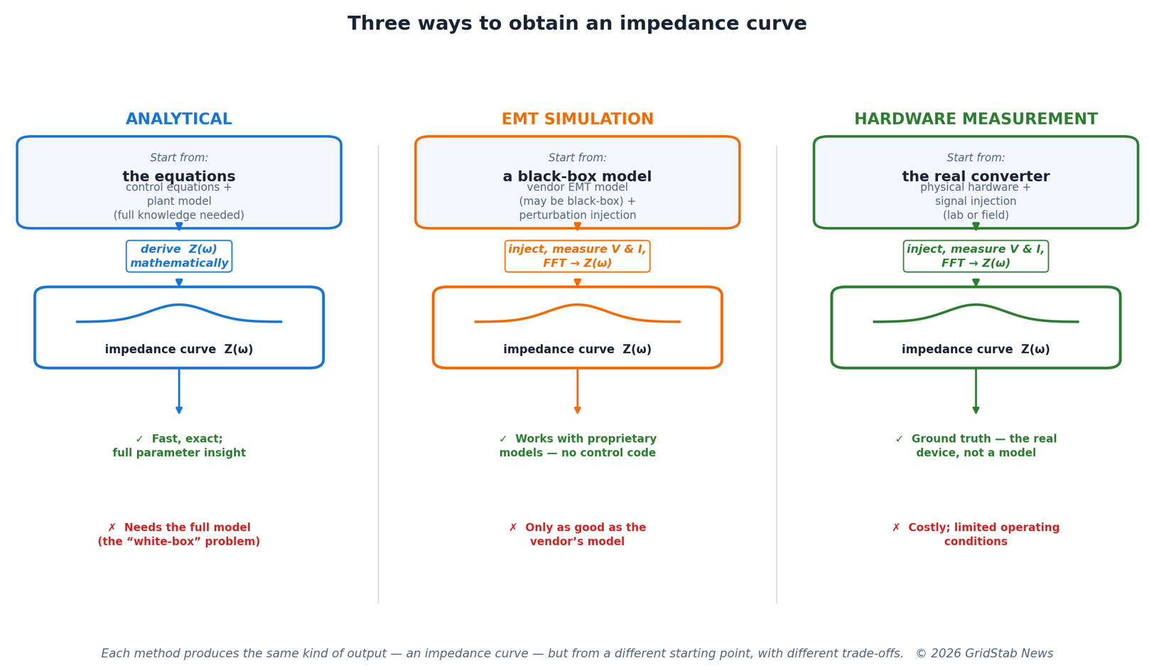
The first is analytical derivation. If you have access to the complete mathematical description of the device — its control equations, its power-stage model, its filter parameters, and its delay structure — you can derive the impedance algebraically. The resulting expression is exact, fast to evaluate, and gives direct insight into which parameters drive which features of the impedance curve.
The second is EMT-based frequency scanning. You take the device’s electromagnetic transient simulation model — the kind of model that vendors provide to TSOs for connection studies, often as a compiled black box — run it at a specific operating point, inject a small perturbation at a chosen frequency, record the resulting voltage and current, and compute their ratio via Fourier analysis. Repeat at each frequency of interest, and the impedance curve builds up point by point. The scan does not care what is inside the model. It reads the impedance from the outside, exactly as Article 2’s perturb-and-measure principle described.
The third is hardware measurement. You connect the real physical device to a test rig, inject perturbations using a power amplifier or a dedicated measurement inverter, record the terminal voltage and current, and process the signals exactly as in the EMT case. The result is the ground truth — the impedance of the actual hardware, not a model of it.
All three methods produce the same kind of output: an impedance curve, Z(ω), as a function of frequency. In the ideal case, all three would agree perfectly. In practice, they do not. Understanding why, and knowing which to trust in which context, is one of the most important practical skills in impedance-based stability assessment.
— YOU ARE ~30% INTO THIS ARTICLE —
What follows behind the paywall
● Analytical derivation in depth — what it gives you, why it requires the “white box,” and the situations where it remains indispensable.
● EMT-based scanning step by step — single-frequency sweep versus broadband PRBS injection, what the dq-frame complicates, and how automated scan tools work in practice.
● Hardware measurement — how physical impedance tests are performed, the injection devices used, and the practical limits of field measurement.
● When the three methods disagree (with comparison diagram) — why they diverge at high frequencies, which to trust at each stage of the connection process, and the BorWin1 callback.
● What this means in practice — the typical workflow from design to commissioning, and the deeper structural limits that set up Article 6.
Subscribe to GridStab News to unlock the full article and the rest of the series.
